In this post I will make the argument that error control (feedback) is not sufficient for good planning and that feedforward control is indispensable for good planning. To understand my motivation around this it is necessary to take a detour and talk about co-simulation, cyberphysical systems and my work on FmiGo. This post may seem meandering and in a sense it is, because it touches on some interrelated concepts.
Co-simulation and cyberphysical systems
Co-simulation revolves around coupling simulators written in different toolchains. A company like Scania that manufactures trucks will have different departments working on different parts of a truck. Each of these departments use different simulation toolchains for the parts that they develop. The engine department might use one toolchain to do its simulations and the chassis department might use another. Without some way to couple the simulations, each department must use a simplified model of the other departments' parts. The idea of co-simulation is that each department's actual simulator is used as part of the simulations carried out by every other department. The goal is to run all simulators as a whole, despite each simulator having its own internal solver. Another example where co-simulation is desireable is when splitting up simulations for parallelization. This turns out to be non-trivial for reasons that I will get to.
Cyberphysical systems are systems that feature these kinds of simulators but where real physical systems can be plugged into the loop, such as an engine in a test cell coupled to a road model and a driver model. A planned economy is such a cyberphysical system. Another example is a human operator interacting with a simulation, also known as human-in-the-loop (or, humorously, monkey-in-the-loop).
FMI
The Functional Mock-up Interface (FMI) is a standard for wrapping simulators like those described in the previous section. Each such simulator is called a functional mock-up unit (FMU) in FMI parlance. An FMU is a .zip file with metadata stored as XML and the simultor itself stored as either shared object file (.so, .dylib and/or .dll) or as source code, or both. The simulator uses a standardized API. A master stepper uses this API to exchange information between FMUs and also to step time forward, to save/restore FMU state, to get partial derivatives and many other tasks. Not all FMUs implement all this functionality, which is where part of the challenge of co-simulation starts.
Besides co-simulation, FMI also supports model exchange, where each FMU exposes the system of ordinary differential equations (ODEs) that defines their behavior. All inputs, including time, can be changed at will, and the resulting derivatives read off. This allows the master stepper to integrate all FMUs as a whole. While very useful for accurate simulation, such a model is unrealistic for the behavior of real workplaces (though it may be useful for planning). Co-simulation, where an FMU/workplace is allowed to "do its thing" for a period before communicating again, is a more realistic model.
FmiGo
FmiGo is a master stepper developed at UMIT Research Lab. The work was led by Claude Lacoursière. I entered the project some time after it began and have been maintaining the code ever since. It is free software, and we'd like to see more people use it, so feel free to check out the FmiGo website if co-simulation is your thing.
Co-simulation by example
A concrete example of the problem of co-simulation is keeping the output shaft of an engine FMU locked to the input shaft of a driveline FMU. See the image below.

The engine FMU models the inner workings of the engine, clutch and gearbox whereas the driveline FMU models the behavior of the driveshaft, differential and wheels. There are multiple modes at play in the system that happen at different timescales. Fast modes of the system include the driveshaft and engine internals while slower modes are the behavior of the wheels and the gas pedal.
A system that has a large ratio between its fastest and its slowest modes is called stiff, and the ratio is called the system's stiffness ratio. Stiff systems are notoriously hard to deal with, especially in co-simulation. This is because each system cannot be stepped with a timestep longer than a fraction of the period of the fastest relevant mode. If for example the engine runs at 3000 RPM, the gear ratio is 1:5 and we need 1000 steps per revolution of the driveshaft, then each global timestep cannot be longer than 100 µs. This is a huge amount of overhead. Each simulator can only be run for 100 µs, then data must be exchanged, and only then can each simulator be let loose on another 100 µs. Meanwhile the monkey in the loop only cares about things that happen on timescales around 100 ms or slower. If we didn't need 1000 steps per revolution but instead could get away with say 10 steps, then we only need a much more reasonable 10 ms per global timestep.
Force-velocity coupling
One way to couple the two simulators is to use something called force-velocity coupling.

In the image above the angular speed of the gearbox' output shaft is fed to the driveline FMU, and a torque τ is fed back to the engine FMU. τ is computed by inserting a spring and a damper inside the driveline FMU between the driveshaft and an "immovable wall" or "connector" with infinite inertia rotating with angular speed . In the figure above this is illustrated as a spring and a dashpot respectively, and a small "plate" representing the immovable wall. Those who prefer rotational rather than linear parts may think of these as a clockspring and a hydrodynamic damper respectively.
The damper contributes to the torque proportional to the difference in angular speed, and the spring contributes torque proportional to the difference in accumulated angle, which is computed by integrating the difference in angular speed, like so:
where is the damping coefficient and is the spring coefficient. This is called force-velocity coupling in the literature. τ is fed back to the engine FMU at each global step. One can use (from the driveline FMU) either τ's instantaneous value at the start of the current timestep, the end of the current timestep, or an integrated average over the entire timestep. On the gearbox side, the received τ is typically held constant. Note the similarity to proportional-integral (PI) control.
If the timestep, k and d are chosen appropriately, then the entire ensemble will behave as one would expect. If the truck is driving up a hill, the driveshaft will start slowing down. This will cause a mismatch in angular speed between gearbox and driveshaft which will result in a higher counter-torque being fed back to the engine. The engine will then slow down and both sides of the shaft constraint will eventually converge as the truck finds its new equilibrium speed given the current gas pedal input. The choice of coefficients is non-trivial and depends on the global timestep and the inertia of all parts of the system, both of which may vary considerably.
If and are set too low then the resulting system behaves as if the driftshaft is a highly flexible torsion spring (or a wet noodle). Step on the gas pedal and nothing happens for several seconds as the violation between the two sides of the shaft coupling builds, until sufficient torque develops and the truck finally starts moving. Once the truck does move, the pent up energy in the coupling will cause the speed on the input side of the driveline to overshoot and oscillate, and the system will overall behave as if there's no causal link between the gas pedal and the wheels. An undesired dynamic has been added to the system which is entirely an artifact of the coupling. Me and Claude use the term "pneumatics" for this undesired compressibility, to distinguish it from the incompressible "hydraulic" behavior of the preferred method used by FmiGo (SPOOK) which I will get to.
If on the other hand and are set too high then the system will become numerically unstable and quickly explode. This can be thought of as the system overcorrecting for errors in each timestep.
A final option is to decrease the global time step, increasing the number of times ω and τ are exchanged per second. This degrades performance but can bring the violation between both sides of the coupling arbitrarily low if and and are also increased appropriately.
What is described above amounts to error control. There is no way the system as a whole can anticipate and correct for errors before they happen. Even when errors do occur, it takes a long time for the system to converge to a coherent state. Finally, convergence is linear, meaning the error shrinks as where is the global time step.
SPOOK
The SPOOK solver used by FmiGo achieves quadratic convergence, [1]. It revolves around computing a set of forces at each time step that, when applied, keeps the whole system together. The way it achieves this is by modelling the behavior of each FMU, and through a bit of time travel. Let's start with the time travel.
SPOOK makes use of the ability of some FMUs to save their internal state and to restore it at a later time. It saves the state of all FMUs, holds their inputs constant and steps them one time step into the future. It then reads the velocities of all relevant connectors, and then resets all FMUs to the present time step. This allows the solver to compute the velocity of the future violations of all constraints. In other words, if during the current timestep the truck starts going uphill, this will result in a future discrepancy between the two ends of the shaft constraint in the present example, meaning the shaft constraint itself acquires a velocity in the future. The solver may optionally also make use of the present violations of the constraints, including both the position and the velocity of the connectors. The economic equivalent of this would be to ask each workplace what they will do for the foreseeable future, all else being equal. Any imbalances between supply and demand can then be treated as constraint violations.
The modelling part of the process asks each FMU for partial derivatives of each connector's acceleration with respect to each force input (). This results in a set of mobilities, the inverse of mass, through the Newtonian . The rotational equivalent is , or in derivative form. Because the solver asks for partial derivatives of all connectors with respect to all force inputs, the resulting set of mobilities contain a set of cross-mobilities. A gearbox has a 2x2 mobility matrix, where the off-diagonal elements are its cross-mobilities, which depends on the chosen gear. A differential has a 3x3 mobility matrix. And so on. The economic equivalent of this would be workplaces reporting their technical coefficients, which can be had either via bills of materials (BOMs) or via statistics.
The existence of cross-mobilities allows the solver to "trace" the action of any part of the system on all other parts of the system, anticipating and applying the necessary corrections. This amounts to a form of feedforward control, as opposed to the error control (feedback) used by force-velocity coupling and by the market. Specifically the equation that is solved looks as follows:
On the right hand side, and are the present violation and speed of all constraints, and are the future velocities. and are constants. is a matrix assembled from the mobilities in a way that is too involved to go into here. Finally is the sought after set of impulses that keep the system together. Dimensions can be chosen for the elements of the matrix, the rows of the vectors and the constants such that the dimensions in the equation become commensurate. The impulses are converted to forces/torques by dividing by the global time step:
After this, and and sent to the relevant sides of each constraint. The figure below illustrates how the FMUs are connected to the solver.

For brevity and are not shown.
In the above system, is a 1x1 "matrix" and so the entire exercise seems perhaps a bit silly. Things become more interesting when we have a more granular system like the one below with 7 separate FMUs and 6 shaft constraints:

In this case is a 6x6 matrix with the following structure:
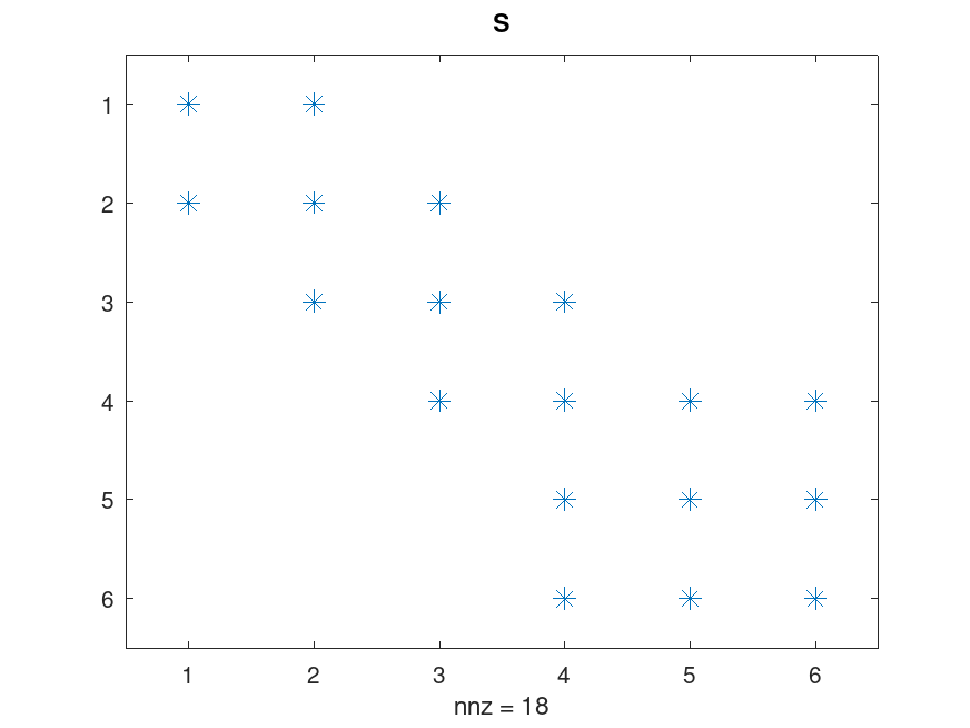
The off-diagonal elements are what ensure that for example increased load on one of the tires are propagated instantly to the engine. The economic equivalent is a change in demand for some final good instantly propagating to all workplaces that supply all inputs necessary to make that good, directly or indirectly. Hence the tug-of-war between consumers and workplaces becomes a hydraulic one, with immediate effects, as opposed to a pneumatic one with delayed effects.
Other solvers/methods for co-simulation
There are other methods for dealing with the co-simulation problem. These include the transmission line model (TLM), Edo Drenth's NEPCE and others. I will not go into these here.
Why does feedforward work so much better than feedback?
In previous sections I pointed out that SPOOK is an instance of feedforward control whereas force-velocity relies on plain old feedback. But why does SPOOK work so much better? The reason it works better is because SPOOK models the system under regulation. In fact any regulator that accurately models the system under regulation will deviate much less from the desired "set point" than a regulator that lacks such modelling. In the examples above the set point is "all constraint violations = zero". In planning we could have "supply ≥ demand" and "supply ≤ environmental limits". More formally, the system's behavior exhibits lower entropy than regulators that lack modelling. Hence modelling is not only beneficial, but mandatory for good regulation. This is the essence of the good regulator theorem formulated by Conant and Ashby[2].
The connection to the market and to planning
Knowing what makes for good regulation, or good cybernetics, and what makes for bad regulation, or bad cybernetics, also allows us insight into why the market behaves the way it does and why the market is so unstable. The market exhibits a number of modes that we call business cycles. Why is this? It is because the market is a decentralized control system, where due to corporate secrecy each part of the system has little idea what the other is doing. In Marxian terms this is called anarchy in production (anarchist readers may prefer the wording "chaos in production"). It is equivalent to the matrix above having no off-diagonal elements. Each workplace is thus forced to resort to error control (feedback). The same is true of any economic system that relies on local control, regardless of the relations of production. In the terminology of Conant and Ashby, this lack of information and coordination results in a high-entropy regulator.
A similar argument can be made against a common appeal to nature, namely that nature is self-regulating. This is true in a sense, but it doesn't mean that nature is a good regulator. Nature is harsh. Take for example the Lotka–Volterra predator–prey model, which is backed by observational data. There are two populations, predator and prey, which oscillate. The predator population lags the prey population by 90°. Without sufficient damping, the predator population will experience periods of extreme starvation. Beyond this being bad for the predators, it also affects humans when said predators start attacking livestock for lack of prey. The prey population, experiencing periods of extreme growth, are also a hassle to humans, as the prey too will eventually encroach on human settlements in search of food. Technically this is a dynamic equilibrium, which is certainly better complete failure, but it is still not good. Examples of even worse regulation in nature include overgrazing by Australian brumbies (wild horses), the Great Oxidation Event and other Great Dyings throughout Earth's existance.
Planning by comparison must take into account how each part of the economy interacts with every other part of the economy, and with the ecology of the planet. This is planning's strength, and also its main challenge.
The unreasonable effectiveness of the Soviet system
The effectiveness of feedforward regulation explains how the Soviet economy could work as well as it did, despite its lack of computational power and despite significant delays in the system due to its pen-and-paper and monkey-in-the-loop nature. It is precisely because demand for goods across the system could be predicted ex-ante that the Soviet system could get away with a large step size. The system was also not as hierarchical as many people seem to think, and in some cases the plan could be partially adjusted surprisingly quickly. According to email correspondence with Elena Veduta, during the Great Patriotic War such re-planning could be done within ten days or so for certain goods.
The good regulator theorem also explains some of the Soviet system's problems. Feedforward regulation can only work as well as the underlying model, which is only as accurate as the data that are given. If the data are wrong, either by deliberate sabotage or by accident, then feedforward cannot function properly. The result is a mismatch between supply and demand, known as imbalance in Soviet parlance. I suspect that even if Gosplan had electronic computers from day one, and even if all data were centralized such that all computations could be done in one place, which would permit perfect balance on paper, this would not guarantee balance in practice. Achieving real-world balance, or the relaxed condition of demand not exceeding supply, is more difficult. This is not news to anyone who's ever built any real-world control system.
Conclusions
My views on planning are influenced by my experience with co-simulation. Black box coordination is difficult, but can be made easier by making the boxes slightly more transparent. We can never make any labour process completely transparent however, because people aren't linear operators.
From Conant and Ashby we know that we cannot dispense with modelling if we are to effect good regulation, where good regulation is taken to mean keeping the system near some set point. For the challenge that faces the human species we could take this set point to be "human flourishing within environmental bounds".
Feedforward control can effect excellent regulation, but only if we have good data. We must quantify the quality of the data we collect. We must provide tools that ease the collection of the necessary data, including automatic sanity checks (gates in Soviet parlance). This data should be accessible to all, which implies logical centralization. In other words, a data commons.
Accounting is the source of much data, which by its nature tends to be of high quality. Therefore we cannot dispense with accounting. We also need information on the use of actual resources, which I posit can be done with in-kind accounting. I plan on writing a text on in-kind accounting in the future, so stay tuned for that!
Finally, because every part of the human economy affects every other part, we cannot rely on the vagaries of human judgement to guide it. Only the blessed machine can ensure orders placed on the production of fuel, lumber, clothes, steel and so on are within global environmental bounds, quickly enough to effect good regulation. The Soviet experience is ample evidence of this. Those who think we can replace computation with meetings must explain whether they think the Soviets were idiots, since they too built their system on a foundation of meetings. One cannot get around this problem by gesturing towards horizontal coordination, since the Soviet system too had plenty of horizontal coordination, as does the market.
References
[1] C. Lacoursière, T. Härdin (2018). FMIGo! A runtime environment for FMI based simulation. Report for Department of Computing Science. ISSN 0348-0542. Fetched 2024-03-16.
[2] R. C. Conant and W. R. Ashby, Every good regulator of a system must be a model of that system, Int. J. Systems Sci., 1970, vol 1, No 2, pp. 89–97. Fetched 2024-03-16.